A summary of how to build a conversion model for a SaaS business using survival analysis and some Bayesian parameter estimation
Background
We need a model to better understand and forecast conversion rates in accordance with the business objectives laid out in this article. Here’s a quick summary:
Users start a free 14-day trial and can convert any time before or after that 14 day mark- but they cannot use the product after 14 days.
We have around 70k observations over a one month period with only the device (i.e. desktop/mobile/tablet) and browser (i.e. Chrome/Safari etc.) on which the trial was started, the timestamp of trial start (in UTC), and the timestamp of trial conversion.
There have been two new features launched during this one month observation period.
Our objective is to develop a baseline understanding of conversion rate in order to better forecast how a major new product launch may impact conversion. This requires first an understanding of the current conversion rate then careful tracking towards our goal after launch.
Understanding the Baseline
To avoid this article being way too long here’s a quick summary of our exploratory found in the notebook linked above:
The rate of trails is seasonal on week but conversion rate is constant.
Users on desktop devices are more likely both to start trials and to convert to paid subscriptions.
Because 99% of all subscription events are observed before day 120 and this corresponds with being exactly one quarter, business’ preferred time frame.
We want to group our users into cohorts since this is the bedrock of survival analysis and will able to quickly assess impacts over time which after all is what we’re doing here.
Conversion rate as a survival curve
Modeling conversion rate over time
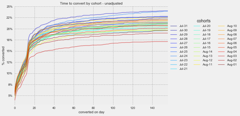
Dealing with measuring an event happening to an observation over time is the foundation of survival analysis- specifically measuring survival: if an event has happened by time t and hazard: the likelihood of an event occurring at time t. If we divide our observations into cohorts (defined by the date on which they started their free trial) and plot the cumulative number of observations we get a plot like the one below which then can be fit to a curve using the Kaplan-Meier estimator.
But wait! We know that different devices convert at different rates! We need to adjust our curve to take into account the variance caused by significant features. We could plot three different KMF curves but this could get tedious as the number of features grows and is more difficult to represent concisely. Instead let’s extend our univariate KMF estimator from above to accept features by leveraging Lifeline’s awesome survival regression modules- namely Cox Proportional Hazards (cph) and Aalen’s Additive model, to adjust our conversion rate for the features.
Survival regression
First of all- both models- CPH and Aalen’s endogenous variables are hazards at a specific time ℎ(𝑡|𝑥). This is the likelihood that a free trial will convert at time t, not will have converted by time t. That sounds pedantic but it is not the same and switching from one to the other requires more calculus that I’m prepared to do right now. Fortunately both methods in Lifelines have a survival curve forecast (which we invert since we want to know how many have had the event happen rather than how many have not i.e. how many are infected not how many are still susceptible).
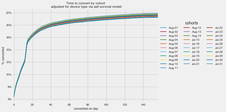
The conversion rate by cohort plot from above after adjusting for device type at trial using Aalen Additive regression model .
CPH is more well known and has slightly better built in tools with lifelines but it assumes proportionality- i.e. the those on desktop don’t convert sooner than those on mobile, the ratio of the chances of conversion (the hazard) are proportional. If our data aren’t proportional we have to address these issues with an accelerated failure parameter.
Aalen’s is simpler and more intuitive. It doesn’t have any of these hangups about proportionality. It also has the added bonus of looking a lot like linear regression [ h (t | x) = β0(𝑡) + β1(𝑡)𝑥1 + ...+βn(𝑡)𝑥n ].
We’ll start with Aalen’s but will leverage some of Lifeline’s cool plots and methods from CPH. If in the future we are able to validate assumptions about proportionality and find significant lift we can switch to CPH.
Forecasting the 120 day conversion rate at time t
The estimated conversion rate for a cohort at day 21- notice we plot only what we’ve observed through day 21 then fit our model to describe the number of conversions after day 21.
Let’s use our model to answer the slightly different question “how many more users are likely to convert?“. Or more succinctly: ĉ(t) 𝚷 ( c(t) / n(t) ) with c(t) as the count of those converted at time t (the ‘infected’) and n(t) as those remaining (the ‘susceptible’) . This requires to make a proportionality assumption- basically that even if our new product does meaningfully impact conversion it does so in a way that does not impact the rate at which people sign up. i.e. if 10 or 1000 people convert on the first day we can still expect each to be roughly 25% of the total conversions by day 120.
This is important as it allows us to make an inference as to the eventual conversion rate every day after trial start and for that inference to become more accurate over time. Now after our product launches we can say things like “this cohort on pace for an eventual conversion rate of x%“.
** Thanks to the model’s roots in epidemiology we have to put up with the terrifying terminology to measuring the hazard to a susceptible population after counting the infected. Because we’re setting the key result for a SaaS business not a cholera outbreak be sure to use friendlier language when presenting findings. This enables us to build a plot like what’s on the right for any cohort at any given time after trial.
Calculating a change in conversion rate
Now after the product has launched- do we notice a change? Let’s walk through how we can answer this over each day of the product launch.
Day 1
Of all the trials that signed up the first day after a product launch- 5.0% of them converted to a subscription. We know from our curves above this corresponds to about a 20% conversion rate by day 120 (we are putting some blind faith in our assumptions here!). This is slightly below the average but this is the equivalent of tossing a coin 1000 times and getting 51%- hardly a smoking gun. Instead let’s put our Bayesian hats on and plot both the first day’s conversion and the historical first day conversion rate as beta distributions. This makes it easier to see just how arbitrary this number is. We can (and should) use a quick chi squared test to assess the significance of this relationship but we can also use the Bayesian approach where we essentially compare the integrals of the curves of our beta distributions to understand the relative likelihood the new cohorts are actually above, below or the same as our historical. This gets us the much more intuitive histogram on the right. This is, in my experience, the most comprehensive way to explain “we don’t know yet“ to stakeholders.
Day 1 summary: We need a few more days to know for sure but right now there’s essentially no change.
Day 7
It’s been a week and we now have more information- both more cohorts starting trials and more days over which to observe them. If we just plot what we’ve seen so far against the baseline we get a kind of hard to read graph but a few things stand out: mainly that first cohort we’ve observed is not doing great but all those thereafter are doing at or above the baseline. If we use our survival model from above to get us an eventual conversion rate for each cohort, then average those to get an overall eventual desktop conversion rate of 23%. Using our plots from above we can see that we’re starting to see a significant positive impact in conversion! Our Chi Squared test returns a significant result at the 95% confidence interval and we can start to feel better about the impact.
Having enough time to tell if the cohorts before and after this launch are significant should also give us enough time to check our assumptions. I’ll leave this to the notebook but some things to watch out for:
Is the device mix consistent?
Is the conversion rate of devices consistent relative to one another?
Do cohorts after the new product launch exhibit proportionality relative to the cohorts before the new product launch?
Day 14
Now the impact is clear and we are starting to develop a more refined understanding of the product launch.


